
The production function relates inputs to an output using a particular production process. The best way to learn about the relationship between inputs and output is to use a specific example where we can visualize the actual inputs and output. Let’s start with a very small agricultural example: a garden.
The output is going to be potatoes. We could measure the quantity produced by the pound, bushel, or kilogram, or even by the individual potato. In any case, the potato will be the product (Q) also known as output.
The inputs are known as the factors of production. What are the inputs we need to grow or produce potatoes? The first, and perhaps most obvious is land. We also need seed potatoes (technically tubers) to start the crop. And how does the crop get planted? Labour. We need people to plant the crop, and once it’s established, we need people to hoe the hills and eventually, to harvest the potatoes. We might also need fertilizer, insecticides for pests, and perhaps herbicides to keep the weeds down, but we won’t worry about that at the moment. In terms of machinery or capital, we likely need a shovel or spade for planting and harvesting, and a hoe for hilling.
The goal of this exercise is to determine how changing the amount of only one input will influence the output. To do this, we are going to make several simplifying assumptions. First, we will hold all of the other factors of production constant and look only at one input and how it affects production. This is known as ceteris paribus, and is used frequently in the study of economics meaning, “other things equal.” This allows us to examine how only one thing at a time will influence or change an outcome while holding other inputs constant or fixing them at a certain level.
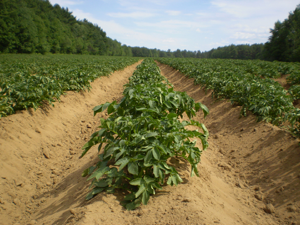
Figure 4.2: Potato Crop. Source: http://www.publicdomainpictures.net/view-image.php?image=23599&picture=potato-fields. Permission: Public Domain.
Let’s assume that land is fixed. Our potato plot in the garden is 5ft x 5ft (or in metric, approximately 1.5m x 1.5m). Let’s also assume that labour is fixed at one person and that for capital we have one hoe, and one shovel. We will now look at the relationship between seed potatoes (one tuber per hill), and the output, actual potatoes.
When we plant no seed potatoes (input = 0), we will get no output (Q = 0, which is the first point on our chart below). When we plant two seed potatoes our output is expected to be nine potatoes. At five seed potatoes, the output grows to 45 potatoes and so on until we have the maximum output at 282 potatoes from 16 seed potatoes. You’ll also see that at 17 hills, the total number of potatoes doesn’t change – it remains at 282.
The graph below maps the relationship between one input (seeds) and one output (potatoes). Input is mapped on the x-axis and ranges from 0 to 20. The output (numbers of potatoes) is indicated on the y-axis and goes from 0 to 300. Each point shows the relationship between input and output. Keep in mind that all other factors of production are fixed (one person, one hoe, one shovel, and the size of the garden).

Figure 4-3: Total production of potatoes (production function). Input is seed potatoes, output is potatoes (#), and other inputs (land, labour and capital) are held constant. Permission: Courtesy of course author Hayley Hesseln, Department of Agriculture and Resource Economics, University of Saskatchewan.
Notice two things in the graph above: that the production function is not straight, and that it starts to decline after input reaches 16. Why is that? Remember that we are holding all our factors of production constant, except for one input, seed potatoes.
When we examine the graph we note that the production of potatoes starts to increase as we plant more seed potatoes and that it increases at an increasing rate. We call this, increasing returns to scale. This means that output is increasing proportionally more than input. This happens right up to the red marker on the graph. After the red marker in Figure 4-3, known as the inflection point, we note that output continues to increase (the total number of potatoes continues to rise) but at a decreasing rate. When output increases at a rate proportionally lower than input increases, we call this, decreasing returns to scale. So, for each unit of input, we will get marginally less output.
Rather than getting caught up in the terminology, consider the story behind the graph. One person is growing potatoes on one small plot of land and has one shovel and one hoe. It’s not surprising that the more hills of potatoes the gardener plants, the more potatoes per hill she will get when they are ready for harvest – this holds true from zero hills to about 10 hills. Each additional hill will produce increasingly more output because each plant is using space in an optimal way.
Of course, the gardener is limited by the size of the garden, and the tools she has. If our gardener were to plant more than 10 hills, they would start to compete for nutrients and produce fewer potatoes per hill.
At the top of the graph where the input is greater than 16, some of the plants might die because they are crowded resulting in a smaller total number of potatoes to harvest at the end of the season. The result will be a decline in the production function showing that the total output actually falls (see the black markers on the graph).
The shape of the curve is a result of how inputs are used together. Many of you come from agricultural backgrounds. You will have seen how the total amount harvested (output) is dependent on the inputs (largely, machinery, labour, and the size of the field). Let’s take another example using wheat harvest, which requires trucks, and combines, and people to operate the machinery.
If the farmer is working alone, he has to drive the truck to the field, let it sit idle while combining, offload the grain to the truck, and drive the grain to the terminal while letting the combine sit idle. There is only so much grain that could be harvested using one person, one truck and one combine. If a second person comes to help, neither piece of machinery has to sit idle and the quantity of grain harvested will increase substantially – the production process will be more efficient because there is no waste. If a third person comes to help, we have the same inefficient situation: labour will sit idle because there is not enough capital to match each person with a piece of machinery.
This relationship is true for almost every production scenario imaginable. Consider a restaurant where the owner has to decide how many people to hire. The property size is fixed (one restaurant with a seating capacity of 30 patrons). The equipment is fixed in the short term (grills, fryers, tables/chairs, salad bar, etc.). The number of people to hire could be mapped where the number of meals served was the output. At zero staff, the production would be zero. If one person were hired, they would have to greet and seat the patrons, take food orders, cook and serve meals, take payment, and then clean up. Jumping to a staff of five, you might have a host, a cook, two servers and a bus person, meaning that the number of meals served was much greater than one could serve. The operation would be more efficient because no time would be wasted as a result of one person having to repeatedly switch jobs.
If we continue the scenario to 10 staff, we might increase the output, but at a decreasing rate of return. We could add a bartender, three more waiters, and another dishwasher. Taking the example to the extreme, if we hired 20 staff members, we would have so many people with nothing to do, they would likely get in each other’s way, gossip around the bar, and decrease the total number of meals served.
Provide two examples of how inputs are combined and what the likely effects are on output.
The production process can be illustrated graphically with one input and one output, as was depicted above, and of course, mathematically, which enables us to evaluate more complex production scenarios. For now, we can look at another example using a table with actual numbers. We will also introduce new concepts that will give us more production information.