
Let’s take a veterinary example that involves vaccinating animals. In the following case, we are going to hold constant the number of animals, the size of the barns, and medical equipment. What we want to look at is how changing labour (input) will increase the number of vaccines administered per hour (output). The table below provides the relationship between input and output, and includes two new pieces of information.
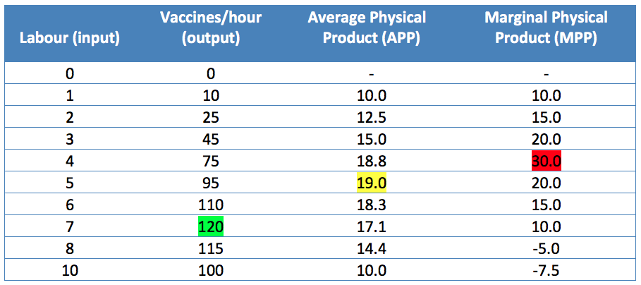
Table 4-1: Total physical production: inputs, output, APP and MPP. Permission: Courtesy of course author Hayley Hesseln, Department of Agriculture and Resource Economics, University of Saskatchewan.
Average Physical Product (APP) is a measure of average total production and is simply the total output divided by the input at each point of production.
APP = output ÷ input
In our example, when we hire one veterinarian to vaccinate animals, the output is 10 vaccines per hour. The average is therefore 10 divided by one, which is 10. For three veterinarians, the output is 45 vaccines per hour making the average 15 vaccines (10 ÷ 3 = 15). Notice that the average rises right up until five veterinarians are hired (APP = 19) and then begins to fall.
The Marginal Physical Product (MPP) measures how much each additional person adds to the total. Hiring the first veterinarian causes quantity to increase from 0 to 10. Therefore, the MPP is 10. When we hire the second veterinarian, the addition of one more person means we will have 15 more vaccines completed. The MPP can be calculated as follows:
MPP = (change in output) ÷ (change in input)
MPP = (25 – 10) ÷ (2 -1)
MPP = 15
Note that the MPP rises until five veterinarians are hired (increasing returns to scale), is maximized where input is five, then starts to fall (decreasing returns to scale), and falls below zero between hiring seven and eight people (negative returns to scale). When so many people are hired, production starts to fall because inputs are no optimally combined.
The graphical representation follows with total production depicted in the first graph, and the marginal and average physical product illustrated in the second graph.
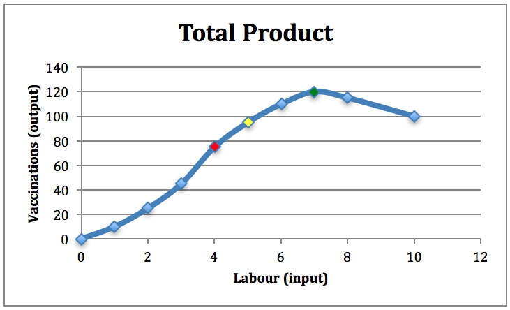
Figure 4-4: Total Vaccinations (input = labour). Permission: Courtesy of course author Hayley Hesseln, Department of Agriculture and Resource Economics, University of Saskatchewan.
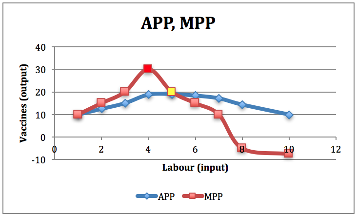
Figure 4-5: Average Physical Product (APP) and Marginal Physical Product (MPP) of Labour. Permission: Courtesy of course author Hayley Hesseln, Department of Agriculture and Resource Economics, University of Saskatchewan.
Some key points to remember.
◊ Maximum total production (in this case input = 7). This is the point where the total quantity produced reaches a maximum. If more labour is hired after this point, production will decrease as indicated by the MPP becoming negative.
◊ Maximum MPP (in this case input = 4). This is also known as the inflection point where we move from increasing returns to scale, to decreasing returns to scale.
◊ MPP = APP, and Maximum APP (in this case input = 5). At this point, the average is at a maximum and also equals marginal physical production.
With the information above, we can now determine the degree to which input affects output (MPP), what our average production is for each unit of input (APP), and the total product possible given the combination of resources we have (those which are fixed or held constant, and the input we are evaluating). Changing any of the resources we were holding constant would change the total output.