
Before you read the next section, watch the video by clicking on the Water Brothers image in Figure 8-5.

Figure 8-5: Water Brothers video regarding water pollution. Source: http://thewaterbrothers.ca/dead-zones/ Permission: This material has been reproduced in accordance with the University of Saskatchewan's interpretation of Sec.30.04 of the Copyright Act.
The Water Brothers are talking about a serious and growing problem – that of nutrient pollution, much of which can be attributed to agricultural production. How does this constitute market failure? Well, nutrient pollution causes damage to the ecosystem that is not accounted for in the market – this is known as a negative externality. Let’s take a look at a market scenario.

Figure 8-6: Negative externality resulting from overuse of fertilizer. Permission: Courtesy of course author Hayley Hesseln, Department of Agriculture and Resource Economics, University of Saskatchewan.
Figure 8-6 shows the market for fertilizer with the regular supply curve (MC) and the demand curve resulting in P and Q, and equilibrium at e. Realistically though, the cost of water pollution and dead zones is not reflected in the marginal cost for fertilizer. That is to say that nobody pays the environmental costs, resulting in overuse of fertilizer – the damage is external to the market. If we were able to measure the value of the damage caused to water bodies as a result of eutrophication, we could add that amount to the MC curve. The new curve would be the marginal social cost (MSC) curve that includes the cost of production plus the value of the damage. That means that we would be producing Q and the marginal benefit would be at e (read from the demand curve), but the marginal cost would be read from the MSC curve at point a. Again, the marginal benefit ≠ the marginal cost and we would have market failure. Furthermore, the blue triangle captures the deadweight loss to society.
The new equilibrium (e*) is optimal because it includes the cost of the damage as reflected by the higher market price (P*) and lower market quantity (Q*). The question is, how do we get there? There are several solutions in this case. First, if we can estimate the value of the damage, the government can impose a tax.
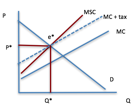
Figure 8-7: Tax as a solution to a negative externality problem. Permission: Courtesy of course author Hayley Hesseln, Department of Agriculture and Resource Economics, University of Saskatchewan.
The solution shown in Figure 8-7 shows how the amount of the tax can force the market to operate at equilibrium. At each point of production, a tax is added to create a new curve (the dashed line). This is the marginal cost + tax. Note how the amount of the tax forces the market to operate at e*.
Another solution would be to force production to Q*. If it were possible to determine the optimal amount of output, the government could limit production by forcing companies to produce lower amounts of output. Alternatively, the government could subsidize the producer by offering the exact amount of revenue forgone to entice the producer to lower the quantity supplied on the market.
While we almost always hear about negative externalities, there exist positive externalities. As is the case with the negative externalities, there is market failure because the marginal benefit doesn’t equal the marginal cost. However, the difference is that production is too low. Let’s look at another agriculture example.
Consider a case where a farmer sprays glyphosate on her wheat crop before harvesting to speed up the drying or desiccation process. If it’s a bit breezy, the spray could spread to the neighbour’s wheat field, thus helping the desiccation process next door. In this case, the neighbour receives a benefit that they don’t have to pay for. So, the marginal benefit of spraying is higher than the marginal cost (Figure 8-8). The graph depicting positive externalities shows an external social benefit or a higher demand curve. The marginal benefit plus the social benefit equals the marginal social benefit (MSB).

Figure 8-8: Positive externality. Permission: Courtesy of course author Hayley Hesseln, Department of Agriculture and Resource Economics, University of Saskatchewan.
The equilibrium point “e” is not optimal because the marginal cost associated with Q is not equal to the marginal social benefit (point a). The result is production that is too low and welfare loss to society equal to the pink triangle. The optimal point of production is at e* with a higher price (P*) and higher quantity (Q*). Social benefits occur whenever people incur benefits that they don’t pay for, or where a higher level of production would result in a better social outcome.
The example above could just as easily be a negative externality if the neighbour were an organic farmer and the glyphosate spray contaminated crops. Consider the climate change example below as it applies to agriculture. Heightened amounts of CO2 in the atmosphere result in costs to society. However, they also result in benefits. How can we determine whether climate change is a positive or negative externality? And then how do we figure out how to arrive at the socially optimal point of production?

Figure 8-9: Perspectives on externalities. Permission: This material has been reproduced in accordance with the University of Saskatchewan's interpretation of Sec.30.04 of the Copyright Act.
Externalities are all around us. Governments can regulate the amount produced, specify the type of equipment that leads to less pollution, and use taxes and subsidies to help internalize external costs or benefits. However, there is another way.
In many cases, externalities occur because there are no markets – usually for “bad” things like pollution. The best example today is the evolution of carbon markets. Because nobody owns the atmosphere, polluters can treat it as a dumping ground and emit all sorts of greenhouse gases (GHGs) at no cost. The government can require polluters to pay for a permit to emit GHGs. Permits are “supplied” according to the quantity of GHGs permissible in the atmosphere, and then polluters can “demand” permits. The price can fluctuate and polluters have an incentive to revise production processes to reduce costs and eventually lower the number of permits they need.
Name one positive and one negative externality in agriculture.