
Just as there are factors that affect us as consumers, there are factors that affect producers. Similarly, a price change is endogenous and will cause a movement along the supply curve and a change in quantity supplied (as you saw in the market examples in the demand sections). The factors that we can’t see will cause a shift in the supply curve.
Consider the types of factors in the world that could affect how much a producer might produce or what might entice a farmer, rancher, supplier or manufacturer to enter the market. Let’s first consider the number of suppliers. What happens when more producers or suppliers enter the market? We can expand on our sausage market example above by considering the effect of six more producers, or 10 more or 100. At the same prices, we would get a higher quantity produced simply because there are more producers making sausages. The effect would be a shift in the supply curve further to the right to reflect more products in the market at each price.
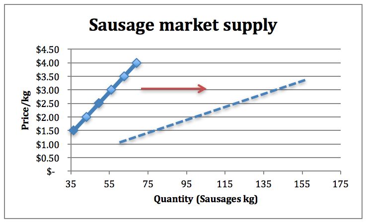
Figure 6-14: Sausage market supply with more producers. Courtesy of course author Hayley Hesseln, Department of Agriculture and Resource Economics, University of Saskatchewan.
Figure 6-14 depicts the likely change of an increase in producers. You see a shift to the right of the supply curve showing that at each price, the quantity available in the market is higher. If producers leave the market, the opposite will happen – supply will fall. (Just a point of clarification here. We are looking at only the change in the total supply without consideration of the other side of the market (demand). Once we add demand there will price changes that follow.)
Think of where this is happening in the agriculture industry. That is to say, where are producers entering (leaving) the market?
According to FiBL, a European research institute committed to organics, there has been significant growth in organic farming with more acres under production and more farmers becoming certified organic. This is a good example of an exogenous change that will result in a shift in the supply curve for organic produce.
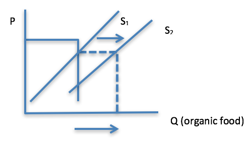
Figure 6-15: Shift in supply. Courtesy of course author Hayley Hesseln, Department of Agriculture and Resource Economics, University of Saskatchewan.
Evaluating the mechanics of the change is much like deconstructing the shifts in demand. In this case, more entrants to the organic market have resulted in an increase in the supply of organic food. Initially, the supply curve shift to the right resulting in an increase in quantity demanded as measured on the x-axis (see the direction of the arrow in Figure 6-15). But we need the other half of the story – demand – to be able to work out the final changes. Let’s look at Figure 6-16 with the demand curve added.
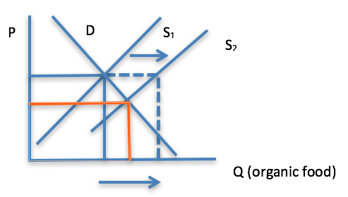
Figure 6-16: Shift in supply of organic foods. Courtesy of course author Hayley Hesseln, Department of Agriculture and Resource Economics, University of Saskatchewan.
We can see now that at the initial price, and the new supply that Demand ≠ Supply. In fact, consumers are not willing to pay the same price to clear the market of the new quantity available. This puts downward pressure on the price to clear the market, which brings the market to a new equilibrium as indicated where D = S2 with a price and quantity that match the orange lines.
Let’s examine another change in the market when producers have expectations about changes to government policy for example. What if you were a cattle producer and expected the US government to relax restrictions on cattle entering the US? Furthermore, you expected this to happen within the next six months. You also know that this would likely reduce your costs because you wouldn’t be required to provide as much documentation. Would you hold back some cattle until later, or sell immediately? The likely answer is that you would sell later because your costs would be lower and we know that means your profits would be higher. In terms of the supply curve, if you and your fellow cattlemen all reacted the same way, we would see a drop in supply in the near future of cattle destined for US markets.
Another factor that would increase total supply (meaning a shift in the supply curve to the right) is when capacity expands. Increasing the size of a farm or production plant would add more to the total supply. Many farms and ranches are expanding and producers are clearing more land for agricultural production. This is particularly true in developing countries where there is great pressure to increase food production and food security to support the growing population.
Producers also have expectations about prices. If they think prices will rise, they might hold back supply in the short term. If they think prices will fall, they might sell right away to ensure higher profits.
Let’s look at the expectation of a price rise. At each price, suppliers will hold back supply thereby reducing the total amount available on the market. The graphical representation will be a shift in the entire supply curve to the left (Figure 6-17). At each price, there will be less quantity available in the market. For example, at a price of $2.50, the quantity offered falls from 50 units noted on the solid line) to 35 as indicated in Figure 6-4 on the dashed line.
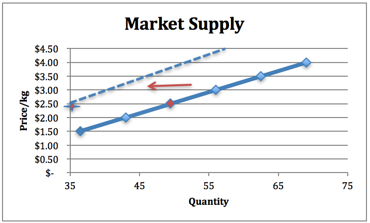
Figure 6-17: Reduction in total supply as a result of higher price expectations. Courtesy of course author Hayley Hesseln, Department of Agriculture and Resource Economics, University of Saskatchewan.
Can you think of something we have not yet mentioned that very much affects agricultural production? If you said the weather/climate, you’d be right! This is true all over the world and good or bad weather can have significant market effects. Rather than looking at another graph, let’s look at the news to see the relevance to our graphs and the effect on supply. In each case, you can click the image, which is hyperlinked, to get the full news story.

Source: http://www.abc.net.au/news/2016-09-02/rain-wipes-out-nsw-crops-in-third-wettest-winter-on-record/7810722. Permission: This material has been reproduced in accordance with the University of Saskatchewan interpretation of Sec.30.04 of the Copyright Act.
The headline above was published on September 2, 2016, in reference to rain in Australia. New South Wales is a state in southern Australia where the weather is typically drier. The overall effect on supply can be illustrated with a shift to the left of the supply curve. The result will be a decrease in price followed by a movement along the demand curve that reflects decreases the quantity demanded.

Source: https://www.sasktoday.ca/south/agriculture/hailstorm-moves-through-weyburn-area-some-crops-wiped-out-5698419. Permission: This material has been reproduced in accordance with the University of Saskatchewan interpretation of Sec.30.04 of the Copyright Act.
In Kansas, this year hail took out part of a wheat crop. The effect on supply would be the same – we could graph this effect by looking at the reduction in quantity supplied at all prices. The supply curve would again shift to the left resulting in higher prices and lower quantity demanded.

Source: http://time.com/4170029/crop-production-extreme-heat-climate-change/. Permission: This material has been reproduced in accordance with the University of Saskatchewan interpretation of Sec.30.04 of the Copyright Act.
The example above looks at crops at a global level and estimates that increased temperatures and decreased overall moisture are negatively affecting crops in the long run. The effect on supply however, is the same: an overall reduction in total supply (shift to the left of the supply curve from S1 to S2 in Figure 6-18). In this case, the supply might be a measure of world crops. Prices increase and quantity demanded/supplied decreases.

Figure 6-18: Reduction in supply as a result of crop failure due to inclement weather. Permission: Courtesy of course author Hayley Hesseln, Department of Agriculture and Resource Economics, University of Saskatchewan.
And, to show that all is not bad in the world, the weather can also produce positive economic outcomes. In the case of peaches, hot weather resulted in a larger crop in Montana. The higher supply of peaches could be illustrated by shifting the supply curve to the right.

Source: http://mtstandard.com/news/local/peaches-in-paradise-hot-weather-produces-bumper-crop-at-forbidden/article_fe9ab02a-c764-5397-9fb8-2b0c30ee10e8.html. Permission: This material has been reproduced in accordance with the University of Saskatchewan interpretation of Sec.30.04 of the Copyright Act.
Other factors that will result in a shift in the supply curve include changes in technology that increase production (precision agriculture, GMOs, drones, etc.), and any government initiatives that positively or adversely affect the cost of production (e.g. taxes and subsidies). In general, anything that influences production will affect the supply curve. We will examine these in more detail in the next module.