
Let’s now make a link between Module 5 and this module by thinking about costs. Each producer incurs costs to make or produce their product. If you are from a farm, you know that your family must buy equipment and other inputs such as seeds, fertilizer, and chemicals (herbicides and insecticides) to grow and harvest crops profitably. If your family operates a cattle ranch, you have to pay for veterinary services, feed, barns, fencing and a whole lot more. If you are in the business of food production, you must buy ingredients for baking or cooking, kitchen appliances including ovens, stoves and refrigeration, plus a whole lot more. In all cases, the producer must incur costs to produce goods that are then sold in the market. Each individual or business/firm faces costs as expressed below in Figure 7-1.
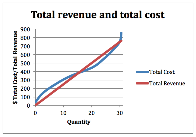
Figure 7-1: Total cost in blue and total revenue in red with price. Permission: Courtesy of course author Hayley Hesseln, Department of Agriculture and Resource Economics, University of Saskatchewan.
By now, this cost curve should be familiar. We could look at this as the costs an individual producer faces or the industry as a whole. In any case, the curve shows that as the producer makes more output, the cost of production increases (see Module 5). Remember now from Module 1 that one of the principles was that rational people think at the margin. We can take a marginal look at costs by asking at any stage of production, what is the cost for making “one more unit?” This is known as the marginal cost.
To determine the marginal cost, we would calculate the change in cost at each stage of production to produce one more unit. This is the change in cost divided by the change in quantity. If we consider changing quantity by one unit, then the marginal cost is the change in total cost divided by one.
For example, if you were a company that manufactures GPS devices for precision farming, you could determine the cost of making the first unit using the analysis we’ve explored up until now. You could ask the question, what would it cost to make a second unit? A third unit? You are asking a question at the margin – what is the cost to produce one more unit?
To calculate the marginal cost, we divide the change in total cost by the change in inputs. It is possible to calculate the marginal cost for increasing production by more than one unit where the move from Quantity1 to Quantity2 is greater than one unit. We could also estimate marginal revenue. That would be the change in total revenue divided by the change in quantity.
MC = (TC2-TC1)/(Q2-Q1) MR = (TR2-TR1)/(Q2-Q1)
Another way to think of the marginal cost and marginal revenue is the measure of the slope of a line tangent to the total cost curve (for marginal cost) or total revenue curve (for marginal revenue). We could also use calculus, by differentiating total cost with respect to quantity or total revenue with respect to quantity. Each method produces the same results and measures the change in cost or revenue as production increases in small increments.
To graph the relationship between marginal cost and marginal revenue, we chart both against quantity. Figure 7-2 shows dollars ($) on the y-axis, and quantity on the x-axis. You see that the marginal cost falls as factors of production are combined in a more efficient way. The marginal cost is at a minimum at 4 units and begins to rise again. The marginal revenue is flat, which should not be surprising given that the total revenue curve is a straight line. If we were to take the measure of a slope of a line tangent to the curve, it will be the same everywhere. The slope of the Total Revenue will equal the price.
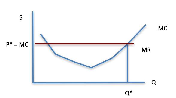
Figure 7-2: Marginal cost ($) and marginal revenue ($) – equilibrium occurs where MR = MC, Q* is the optimal quantity. Permission: Courtesy of course author Hayley Hesseln, Department of Agriculture and Resource Economics, University of Saskatchewan.
The curve in Figure 7-2 is also known as the supply curve (usually we just look at the upward sloping portion). That is to say that the marginal cost curve is the supply curve. Think about this. If you are a producer, and you see the price of the products you make increase, what are you likely to do? Will you grow/make/raise more or less/fewer? The y-axis shows dollars that up until now we’ve discussed as cost. We could also view this scale as price. When the price of a product rises, producers have an incentive to make more. When this happens, you will see a movement along the supply/marginal cost curve. The reverse is also true. When prices fall, producers will make less, or produce fewer units.
You should also take note of where the price line meets the marginal cost curve. This is equilibrium and is determined by demand. Let’s clean up the graph and show you that it is identical to the market graphs we were working with in the last two modules (see Figure 7-3).
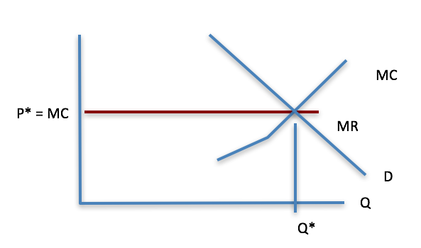
Figure 7-3: Marginal cost and marginal revenue with the demand curve. Permission: Courtesy of course author Hayley Hesseln, Department of Agriculture and Resource Economics, University of Saskatchewan.
We know that the marginal cost curve is the supply curve and that equilibrium occurs at the greatest difference between total revenue and total cost, which happens to be where marginal revenue equals marginal cost. Or, where price is equal to marginal cost. Knowing this to be true helps to clarify some things. Market equilibrium is efficient because, at this point, supply equals demand and profit or rent is maximized for producers. We can look at some other market factors that are important indicators to provide much more information than meets the eye.
Also, you now know how a change in technology or the costs of inputs affects supply. Any enhancement in technology (an exogenous factor affecting supply), will cause the supply curve to shift to the right. Similarly, any decrease in the cost of inputs will also shift the supply curve to the right because the supply curve is the marginal cost curve.