Elasticity

Elasticity doesn’t just refer to what’s holding up your sweat pants. It also measures the degree to which consumers and producers respond to a change in price in the market. It’s similar in that more elastic means a greater stretch or a greater response, and that inelastic means not very stretchy or not very responsive.

Elasticity is very important because it enables us to predict how consumers will react to changes in price for example. We from the law of the demand that if price increases, the quantity will decrease. The question is, how much? If price increases proportionally more than demand decreases, total revenue will increase, which is good for producers. Measuring elasticity will tell us this. Chapter 5 in the textbook provides a comprehensive and detailed explanation of elasticity. I urge you to read the material and visit the links provided in the boxes.

Price Elasticity

Let’s start with your consumption. I’m guessing many of you eat bread – in the form of toast, sandwiches, garlic bread, croutons, and maybe even French toast. The average grocery store white loaf costs what… maybe $2.50 - $3.00? If the price goes up by 15% (which is quite steep), that same loaf becomes $2.85 - $3.45. How much will you change your consumption?

Before you answer that, let’s look at rent. I’m going to assume you are a poor student and that your share of the rent is approximately $500/month. If the price goes up by 15%, what will that do to your rent? It now becomes $575.

Now, you are thinking of getting a new truck (maybe you’re not so poor after all). The price for an average North American-made pickup is $35,000. A price increase of 15% will make the new price $40,250 – a much heftier price hike than for the bread.

In which case are you more likely to change your purchasing decision? Mostly likely for the truck, and for the rent, you might consider getting another roommate.

The change in price for bread, however, is only a matter of a few cents. So, the 15% change in price is not likely to induce a great change in your consumption (change in quantity demanded). The relatively low price of bread combined with the fact that bread is a staple and not a luxury item makes it relatively inelastic. Additionally, the percentage of your income spend on bread is very low compared to the percentage of your income spent on rent.

These factors: low price, a small percentage of income, and being a staple good make food in general inelastic. Now, let’s run the numbers using a simple demand curve.

To measure elasticity we must use the following equation: Because we are working with a straight line, we will use the “midpoint” formula as described in the textbook meaning that we will take the average of two points for the denominator. The formula will look more like this: which says the same thing:

Elasticity = ((change in Q)/(average of Qs))/((change in P)/(average of Ps)).

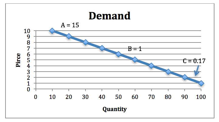
We will calculate three points on the demand curve to arrive at elasticity for each. Assume in each case price is dropping (Figure 7-9).

Elasticity of Point A: = ((change in Q)/(average Q))/((change in P)/(average of P)).

Elasticity of Point A: = ((10-20)/((10+20)/2))/((10-9)/((10+9)/2))

Elasticity of Point A: = (-10/15)/(1/9.5)

Elasticity of Point A: = (-1.5)/(0.10) = -15 → Take the absolute value = 15

Elasticity of Point B: = ((50-60)/((50+60)/2))/((6-5)/((6+5)/2))

Elasticity of Point B: = (-10/55)/(1/5.5)

Elasticity of Point B: = (-.18)/(0.18) = -1 → Take the absolute value = 1

Elasticity of Point C: = ((90-100)/((90+100)/2))/((2-1)/((2+1)/2))

Elasticity of Point C: = (-10/95)/(1/1.5)

Elasticity of Point C: = (-.11)/(0.66) = -0.17 → Take the absolute value = 0.17

At each point on the demand curve we have three different elasticity values. At point A where the price is relatively high and quantity relatively low, the elasticity is 15, meaning very elastic. At point C, the elasticity is only 0.17, which is very inelastic. And, at point B, elasticity is “1” meaning it’s unitary. How should we interpret these numbers?

A point A, we would say for a 1% change in price, we would get a 15% change in quantity. We already know that a decrease in price leads to an increase in quantity – the law of demand tells us this. So, if were to drop the price by 1%, we could expect the quantity demanded to increase by 15%. From a business perspective, would this be a good idea? You bet. The price drop is lower than the increase in demand meaning we will expect revenue to rise.

Let’s look at point C. The opposite is true at this end of the curve because the percentage change in quantity is much larger than the percentage change in price. The elasticity number can be interpreted this way: a 1% decrease in price will lead to a 0.17 increase in quantity. This is relatively inelastic – consumers are not responding very much to a change in price. If producers were to decrease the price at this point on the demand curve, they would lose revenue.

The point in the middle is called unitary elastic because a 1% change in price will lead to a 1% change in quantity, meaning revenue will not change. In general, elasticity can be interpreted as such:

Elasticity > 1 → relatively elastic

Elasticity = 1 → unitary elastic

Elasticity < 1 → relatively inelastic

I heard an interesting story related to elasticity a few years ago, but I’m not sure if it’s true. I was living in the States and it was rumoured that the State government had hit the maximum amount of tax on cigarettes. What I mean is that the government could no longer increase the tax on a good that is typically considered (by smokers anyway) a necessity, and therefore relatively inelastic. Typically, the government will tax those goods because they are inelastic and considered bad for people anyway meaning that an increase in price will result in a smaller percentage decrease in quantity consumed and therefore, more tax revenue. The taxes were high enough that another increase would result in a greater decrease in quantity demanded, and hence, a decrease in tax revenue.

So, if you were ever in a position to increase or decrease prices, wouldn’t it be great to know how your customers would respond before you changed prices? That’s the power of elasticity.

Here’s another great example of the elasticity of organic food:

“The challenge for more specialized organic food companies versus their larger counterparts in many respects comes down to a matter of the elasticity of demand. For while food in general is a broadly defined market that benefits from its inelasticity of demand since people have no choice but to eat, organic food specifically is a narrowly defined market whose demand is much more elastic. This is due to the fact that organic food is more of a luxury item where lower price substitutes are readily available. In short, if economic conditions deteriorate, grocery shoppers can simply forgo higher priced organic food for their lower priced traditional counterparts” (Parnel 2016).

There is a lot packed into the article and the excerpt. You will note that it’s about food, which generally has a low elasticity; and it mentions luxury items (and how they are more elastic), all of which might be influenced by the range of choices and substitutes.

As we discovered above, luxury items are typically more elastic because people don’t need them and can be more responsive to changes in price. Another factor that affects elasticity is whether there are close substitutes. The greater the choice we have, or the higher the number of substitutes, the more flexible (elastic) we can be when it comes to changes in price.

Elasticity Over Time

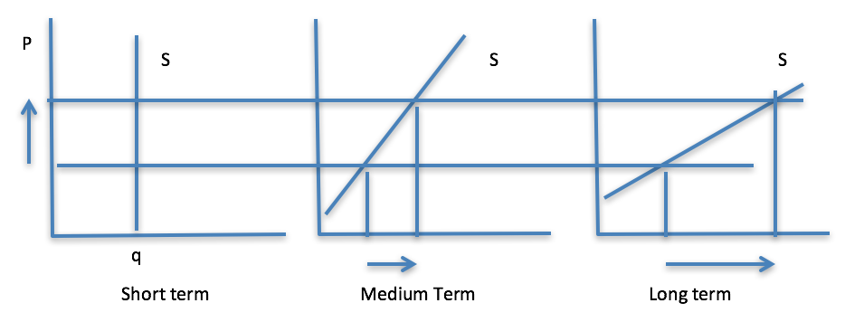
Time is also a factor when it comes to elasticity. Think of the farmer’s market and the supply of produce. Which one of these timeframes (short, medium or long) would represent the market on a Saturday?

For convenience, I’ve used only two prices and haven’t added the shift in the demand curve that would induce such price changes: the low price (the lower line that goes through each supply panel), and an increased price. On a Saturday at the market, the farmer is not likely able to adjust supply regardless of what happens to price. The reason being that the farmer loaded her truck to capacity and has just enough room in the stall for a day of selling. There’s not much that can be done if there is a rise in price (say from overwhelming demand due to good shopping weather). She cannot pick more vegetables and certainly can’t plant more to meet the demand. In this case, her supply is totally inelastic meaning there will be no change in quantity given a change in price.

Let’s define the medium term to be a month. If our farmer were preparing a supply over the medium term and was watching prices, there would be some flexibility in the supply. She could pick more vegetables, load two or more vehicles, and rent bigger space. Her supply would be much more flexible and she could respond. In time the supply cure is no longer vertical showing that as prices changes, the farmer can respond by providing more produce.

If the long term is a year or more, the supply curve is much more elastic, meaning that the farmer can respond greatly to changes in price. She now has the option to expand operations by planting more crops or even buying more land to respond to rising prices. The more flexibility and options the supplier has, the flatter the supply curve.

This is true for both supply and demand. Not only will there be different elasticity associated with each point on the curve, the steepness or flatness of the curve also indicates more or less elasticity. The steeper, the less responsive changes in quantity will be to changes in price, and the flatter, the more responsive to the point where each cure could be flat.

Income elasticity has to do with the percentage change in quantity brought about by a percentage change in income. The calculation is similar to that of the price elasticity of demand → % change in quantity demanded/% change in income.

Similarly, cross-price elasticity looks at the percentage change in demand of one good, given the percentage change in price of another. For example, we could measure the cross-price elasticity for pork given a change in beef prices. The article below discusses the importance of elasticity and cross-price elasticity in terms of government policy.

You’ve likely heard rumblings about taxing sweets and junk food to help improve society’s health and waistlines. This is true in Canada and other countries. If there’s a tax on sugar, the theory is that the increased price will reduce consumption – according to the law of the demand. The percentage reduction in quantity consumed could be estimated if you knew the elasticity. However, there is more than one form of sweetener (or fat, or type of junk food). Might it be possible to switch from one form of “bad food” to another? What do you think the cross-price of elasticity is with other high-calorie foods? Click on and read the following article to find out.